Graph-based network analysis in schizophrenia

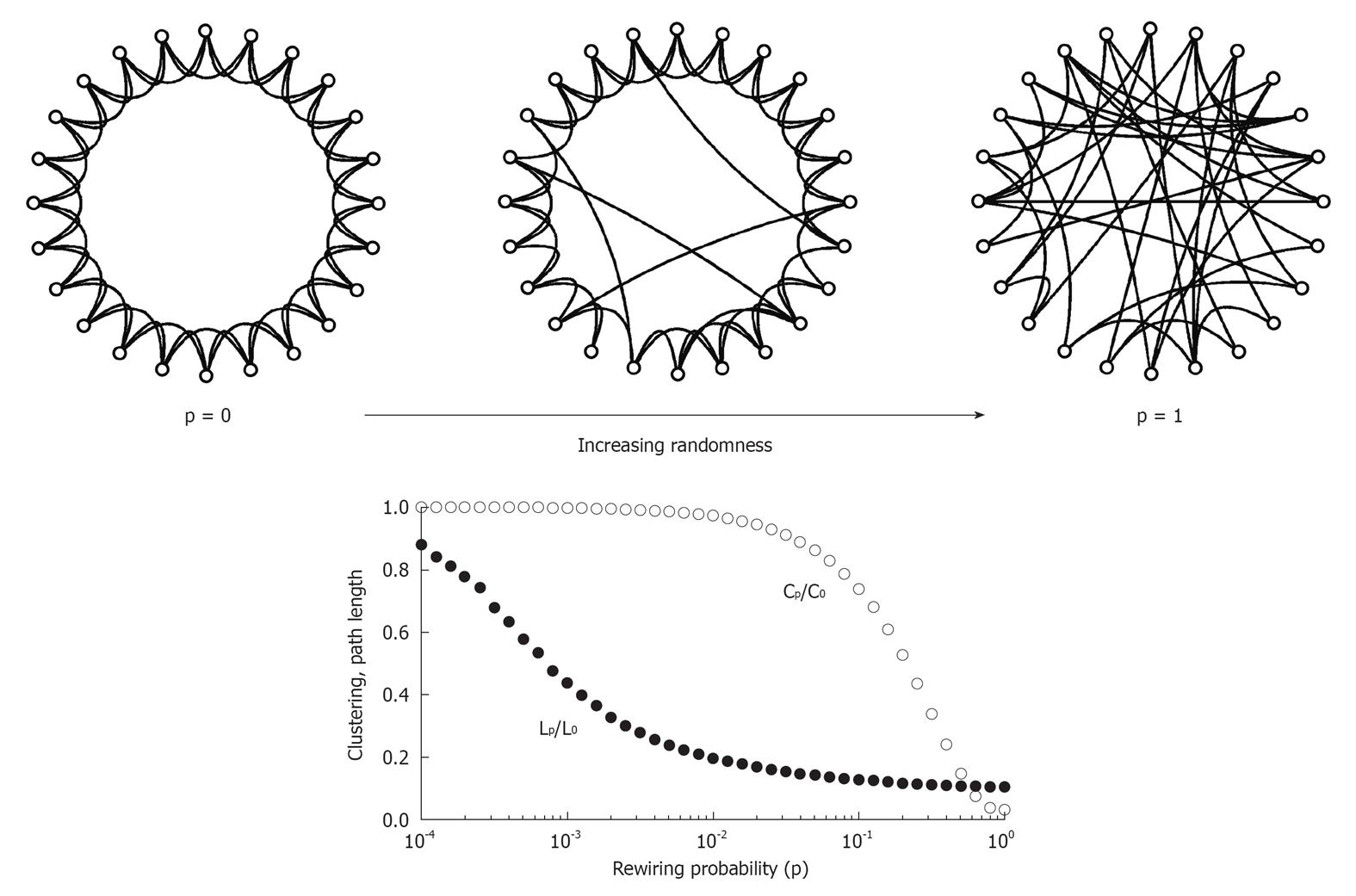
Figure 1 The Watts-Strogatz model of the small world. The network at the upper left corner represents a ring lattice with circular boundary conditions. Starting from this configuration, connections are randomly rewired with given rewiring probability p. For p = 0 (no rewiring), the network retains its regular lattice topology. For p = 1, the network is completely random, and all lattice-like features have disappeared. Intermediate values of p result in networks that consist of a mixture of random and regular connections. The plot at the bottom shows the clustering coefficient Cp and the path length Lp, both normalized by their values for the regular network (P0, L0). Note that there is a broad range for the rewiring probability p when networks have clustering similar to the regular network’s clustering and a path length similar to the random network’s path. Within this range, networks exhibit small-world attributes. Data computed following the procedure is described in Watts and Strogatz (66), with networks consisting of 1000 nodes and 10 000 edges (data points represent averages of 400 rewiring steps)[85].

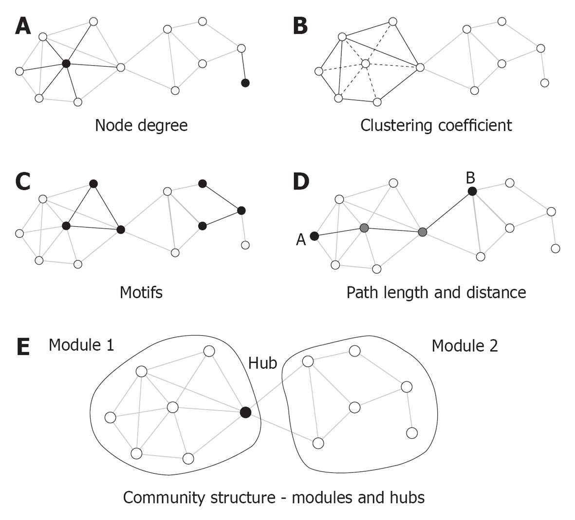
Figure 2 Key graph measures and their definitions. The measures are illustrated in a rendering of a simple undirected graph with 12 nodes and 23 edges. A: Node degree corresponds to the number of edges attached to a given node, which are shown here for a highly connected node (left) and a peripheral node (right); B: The clustering coefficient is shown here for a central node and its six neighbors. These neighbors maintain eight out of 15 possible edges for a clustering coefficient of 0.53; C: Each network can be decomposed into subgraphs of motifs. The plot shows two examples of two different classes of three-node motifs; D: The distance between two nodes is the length of the shortest path. Nodes A and B connect in three steps through two intermediate nodes (shown in gray). The average of the finite distances for all node pairs is the graph’s path length; E: The network forms two modules interconnected by a single hub node[85].

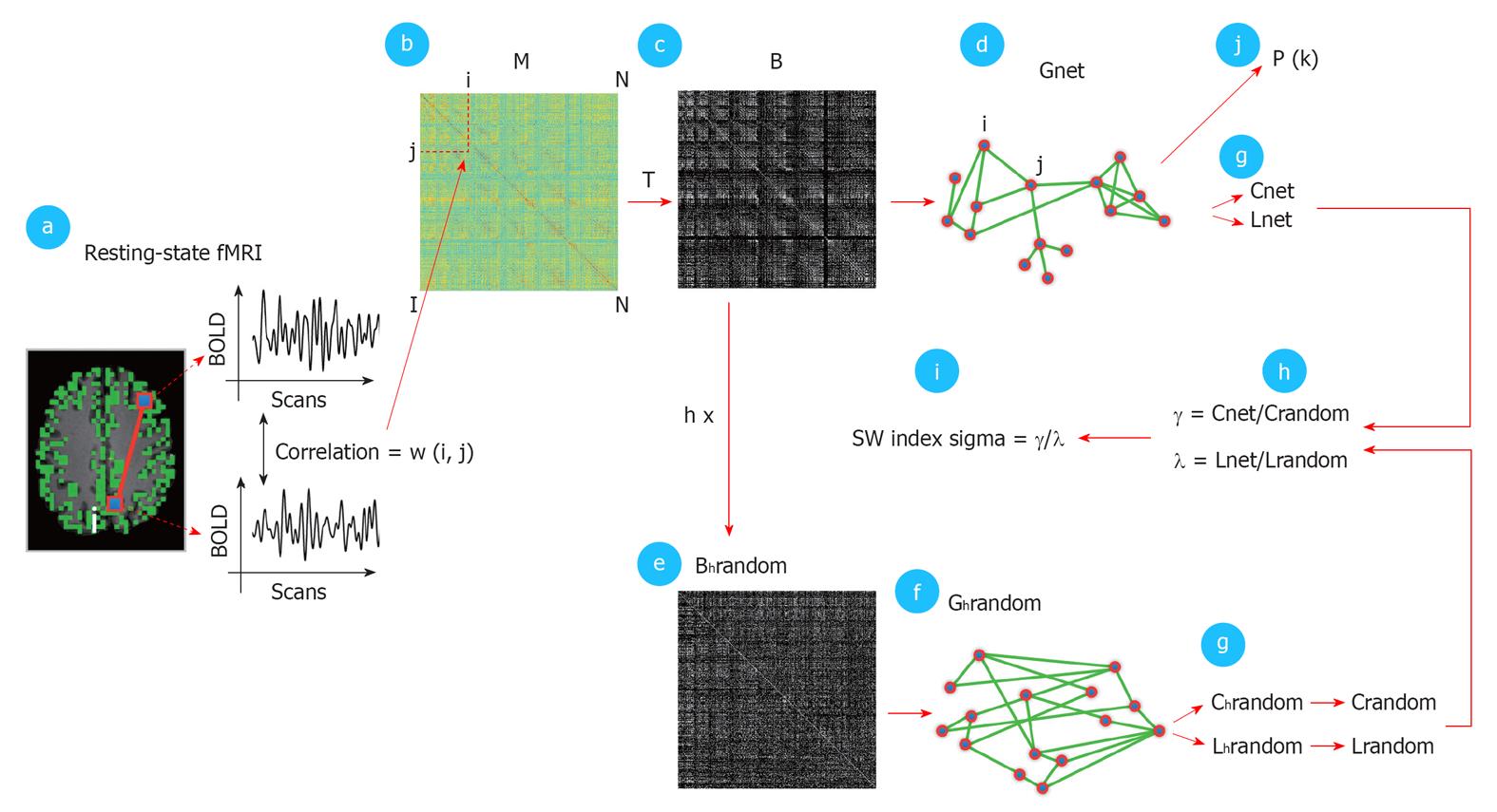
Figure 3 Detailed schematic illustration of the graph analysis. The first step (panel a) consisted of calculating the temporal zero-lag correlations between the filtered functional magnetic resonance imaging BOLD time-series of all voxels, which was believed to reflect inter-voxel functional connectivity. The computed correlations were represented as a correlation matrix M, with cell M (i, j) holding the level of functional connectivity between voxel i and voxel j (panel b). M was thresholded with a threshold T (panel c), resulting in a binary connectivity matrix B, representing an unweighted graph Gnet (panel d). T varied between 0 and 0.7 (with steps of 0.05) and a range of fixed k between 4000 and 20. For each fixed k, M was thresholded with a computed T that corresponded exactly to a connectivity degree of k for that particular individual dataset. Next, B was randomized (panel e) to create a random graph Grandom with a similar connectivity distribution P (k) as Gnet but a random organization of connections. Also, h random graphs were formed per Gnet. From Grandom and Gnet, the graph characteristics Cnet, Lnet, Crandom, Lrandom were computed (panel g). Crandom and Lrandom were created by averaging the clustering-coefficient and path length of the h random graphs. Next, γ and λ were computed, as defined as Cnet/Crandom and Lnet/Lrandom (panel h). The small-world index sigma was computed as the ratio between γ and λ (SW index, panel i) expressing the small-worldness of Gnet. In addition, the connectivity distribution P (k) of Gnet was computed (panel j). Finally, the individually computed graph characteristics were averaged over the group of subjects and the group averaged connectivity distribution P (k) was fitted with a power-law function to examine a possible scale-free organization of the functionally connected human brain[36].

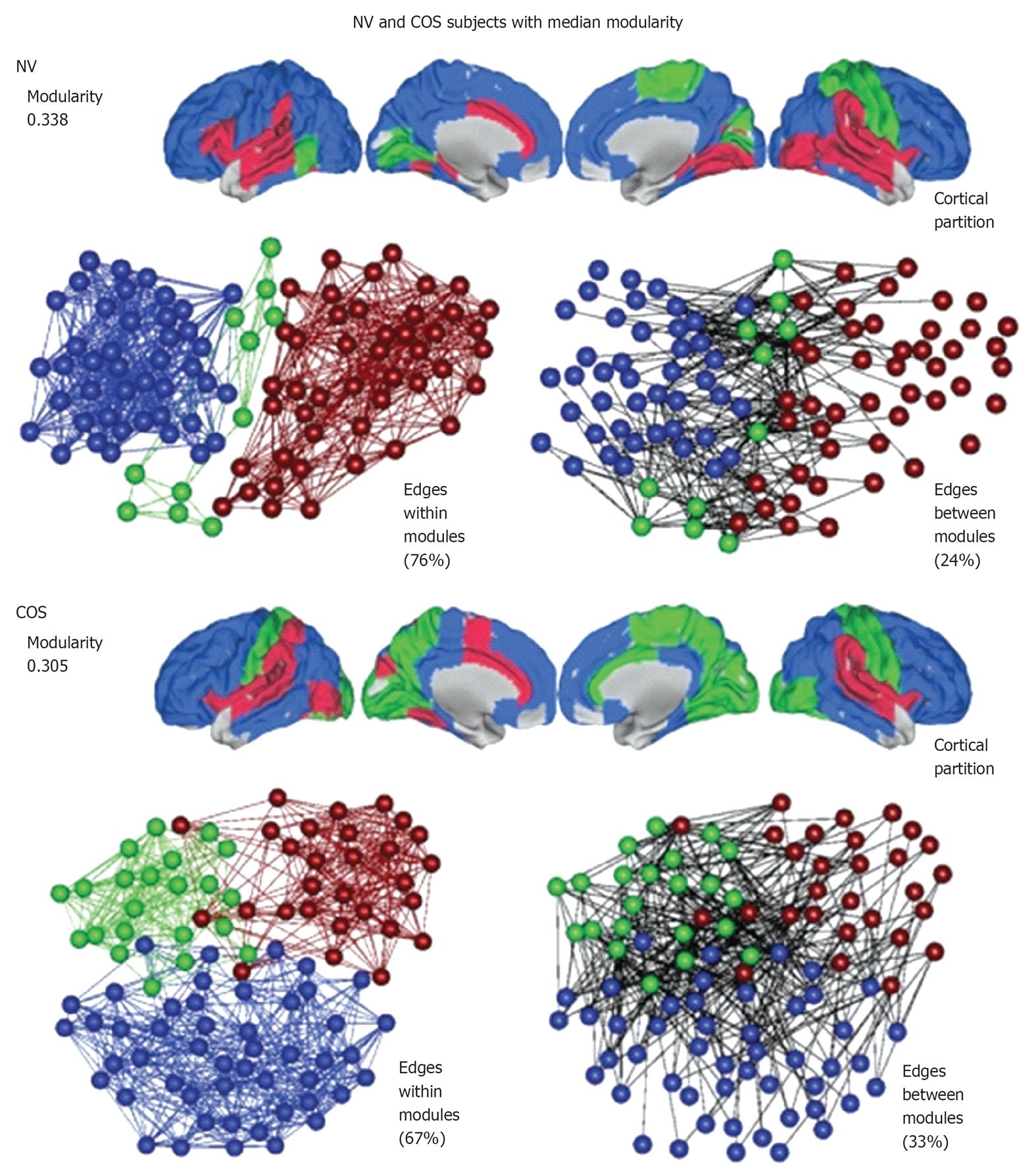
Figure 4 An illustration of modularity using representative brain networks from a childhood-onset schizophrenia population and a control (NV) population. At a local threshold of 0.22 topological cost, the modular partition is shown for the median NV subject (above) and the median childhood-onset schizophrenia (COS) subject (below). Each module is assigned a specific color and the modular structure of each subject is illustrated in three different ways. The cortical partition shows the anatomical location of modules, while the left-hand topological plot shows the density of intra-modular edges between nodes in different modules[69].