Is the pain in chronic pancreatitis of neuropathic origin? Support from EEG studies during experimental pain

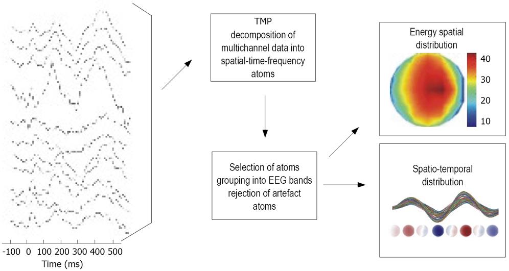
Figure 1 The analysis scheme used for the data investigation. The EEG data were decomposed into a set of TMP atoms, which parameterized the data. Next, the atoms were grouped into bands according to their frequency parameter. This allowed convenient analysis of time and spatial properties of oscillations in all frequency bands.

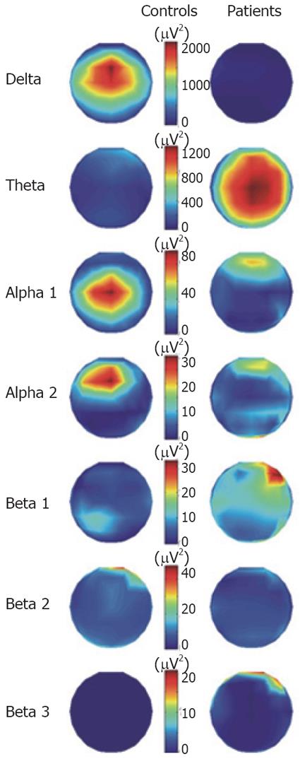
Figure 2 The spatial distribution of energy divided into frequency bands for patients and controls throughout the 450 ms of analysis. Note that a different color scaling for each frequency band was used.

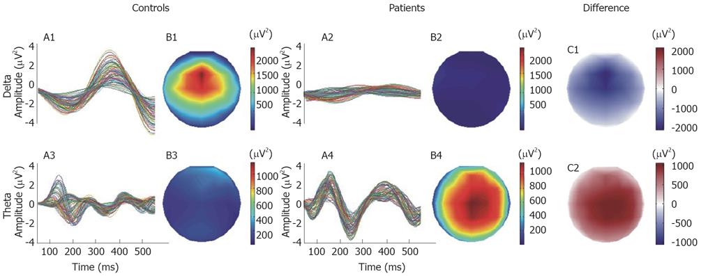
Figure 3 The temporal evolution and the spatial distribution maps of energy of the delta and theta activities for the 450 ms of analysis. In the right panel, the difference maps of energy were computed by subtracting the energy maps of controls from the patients.

Figure 4 The time evolution of amplitude distribution for delta and theta bands in patients and controls. Note the stable, monopolar spatial distribution of delta activity in controls (CD). This is due to constant and small phase differences between measurement channels. The theta activity in patients has slight changes in phase and, therefore, the spatial distribution is not always stable (see arrows). PD: Patients delta; PT: Patients theta; CD: Controls delta; CT: Controls theta.

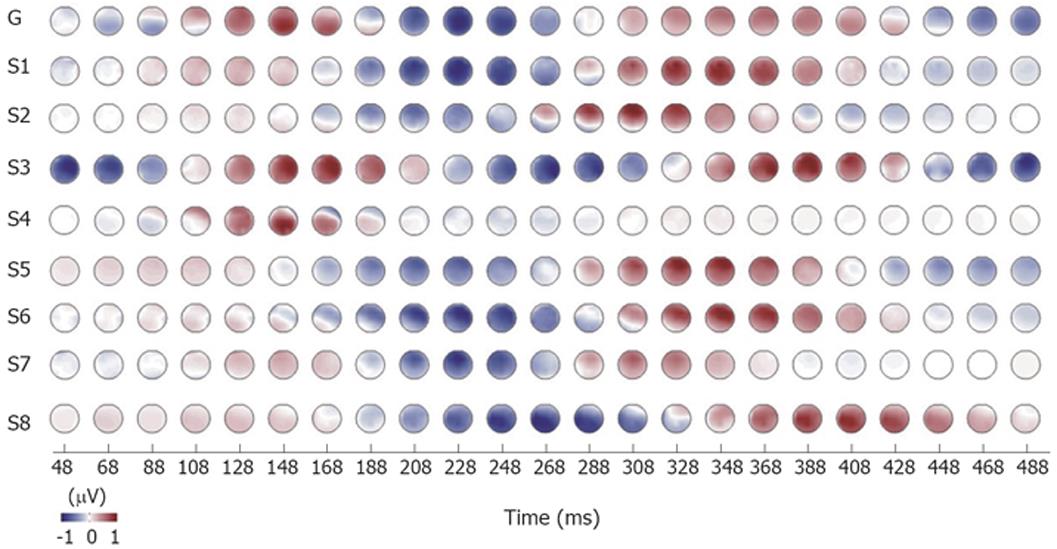
Figure 5 Normalized time evolution of amplitude distributions for theta bands in patients with chronic pancreatitis No. 1-8. G: Grand mean of all patients.

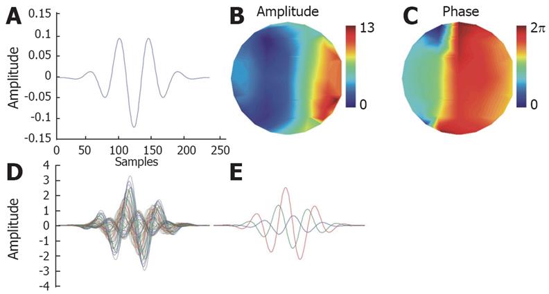
Figure Appendix1 Example of a TMP atom for a 61 channel EEG system. A: Base Gabor atom; B: Spatial distribution of amplitude; C: Spatial distribution of phase; Overlay plots of the TMP atom: All 61 channels (D), channels 1, 10 and 30 (E).

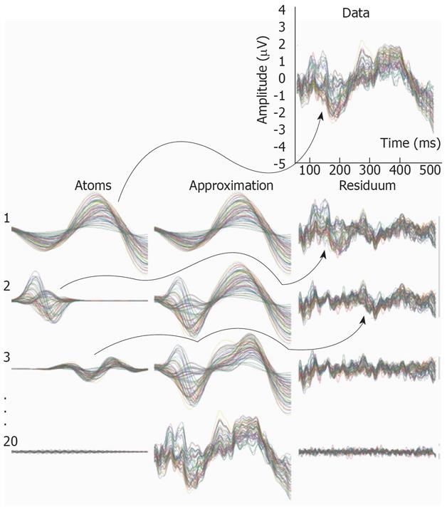
Figure Appendix2 Example of decomposition of multichannel EEG data. The data is presented in the top-right corner (61 channels overlay plot). In the following rows chosen atoms, approximations and residues for the 1st, 2nd, 3rd, and 20th iteration are shown. In each iteration the chosen atom is the most similar one with the previously computed residuum (see arrows). The residuum is created by subtracting the chosen atom from the residuum computed in the previous iteration. The signal itself can be treated as the 0th order residuum. The approximation in each iteration is the sum of all atoms chosen in the present and previous iterations. Hence, in the first iteration the chosen atom is simultaneously the first approximation of the data. Note that with the increasing number of iterations the approximation is approaching the data and the residuum is vanishing. All time plots of atoms, approximations and residues are 61-channel overlay plots shown in the same scale.